DeepLTK Tutorial #2.3: Power Line Fault Classification
- Ish Gevorgyan

- Nov 14, 2023
- 5 min read
Updated: Nov 6, 2024
Introduction
In this tutorial we want to examine a more specific case of waveform classification, specifically classification of faults in transmission power lines.
Power transmission lines connect power generation stations with power consumers in order to effectively transmit large amount of electricity.
There is a high demand on the quality of transmitted (received) power, as poor power quality can result in equipment damage and other issues for both utilities and end-users. To address this, it's crucial to identify and categorize faults like sags, swells, interruptions and oscillatory transients that can appear in transmission lines.
Below are some common types of faults that can happen in power transmission lines.
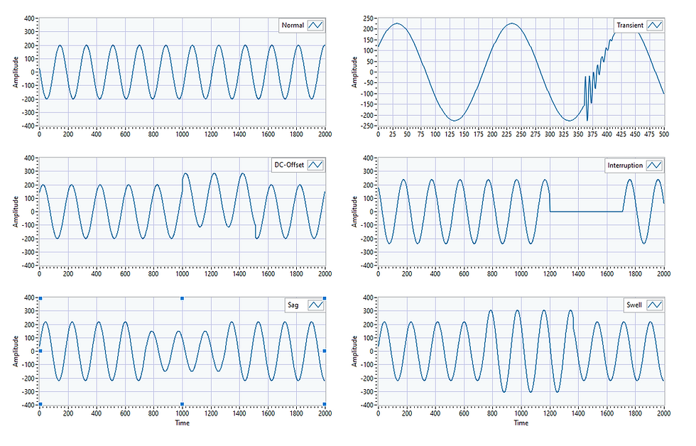
DC-offset occurs after switching non-linear loading.
Sags (or under-voltages) occur when the neutral wire of an electric power system comes in contact with the ground.
Swells and over-voltages are caused by large load changes and power line switching
Transients are initiated due to disturbances like switching, occurrence of short-circuit faults or lightning discharge.
Interruptions occurs when the circuit breaker trips due to overloading.
In this blog post, we'll use deep neural networks via DeepLTK to recognize and classify above mentioned types of faults.
The project is divided into three main segments: Synthetic Data Generation, Training, and Model Deployment. Let's explore each of these in detail.
Synthetic Data Generation

Due to the lack of such datasets available online, we opted to create one synthetically. Below are the details of the dataset generation VI.
The initial step involves generating a synthetic dataset for various fault signals, including DC-offsets, interruptions, sags, swells, and oscillatory transients, along with normal sinusoidal signals. The dataset creation is a two-fold process: the first part generates both normal and faulty signals with variable parameters, while the second part saves generated data samples into .txt files, where each sample (waveform) is stored in separate file.
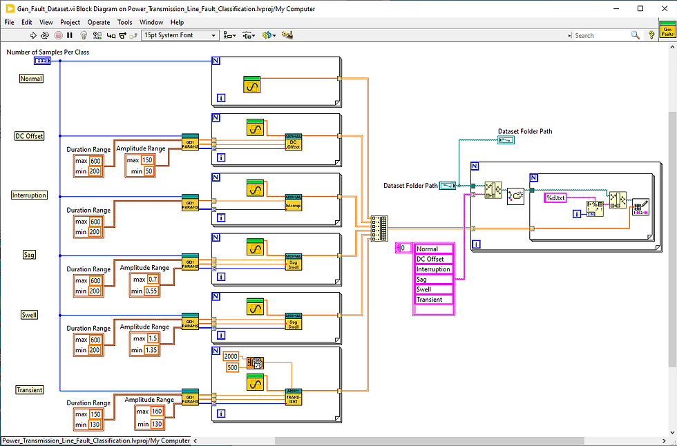

The group of signals of a specific type is stored in a separate folder named after the class of the signal. Specifically here this would be "Normal", "DC Offset", "Interruption", "Sag", "Swell", and "Transient".
These approach of grouping signals into folders later will be used to identify the signals during reading the dataset for training and assigning appropriate labels to waveforms based on the name of the folder containing them.
Additionally, we think that this approach of representing the dataset is particularly useful as real-world datasets often represented in a similar manner and this example can serve as a useful reference for practical applications.

To generate normal signals, we create sinusoidal waves with variations in frequency, amplitude, and phase. Generating normal signals with diverse characteristics is crucial, as power line signals can experience slight variations due to different disturbances while still adhering to the required standards.
To simulate faults, these normal signals are processed through other VIs, which are responsible for introducing sections of waveforms representing specific types of faults.
Later this dataset can be fed to training VI for training a model.
Training:

In the training phase, we'll apply the same classification methods used in our previous tutorials, adapting them to classify power transmission line faults efficiently.
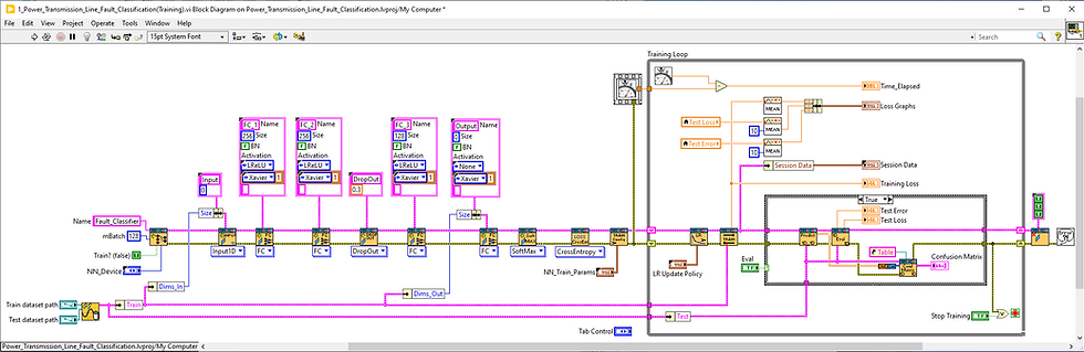
The key difference of this VI are following:
Dataset Reader -
Network model - introducing Dropout layer
Model performance evaluation with help of confusion matrix.
Dataset Reader
The Dataset Reader is designed for user-friendly adaptation to different datasets. Users simply need to organize signals of a specific type into separate folders, with each folder's name serving as the label for that class.

Dropout Layer
The neural network model here primarily consists of Fully Connected (FC) layers. Following the second FC layer, there is a Dropout layer.

Dropout is a regularization technique used during training, where the layer randomly ignores or drops some of the layer outputs (activations). The main parameter of this layer is the "Probability." A probability of 0 implies no dropout, whereas 1 indicates that all outputs of the previous layer will be dropped, i.e. set to zero. In our specific case, the Dropout probability is set to 0.3, which means that only 70% of the outputs from the second FC layer are retained.
Confusion Matrix

The Confusion Matrix is a fundamental evaluation metric, not only calculating but also visualizing the dissimilarity between the network's predictions and the actual ground truth. This matrix helps evaluate the true positives, false positives, true negatives, and false negatives, offering a comprehensive understanding of the network's efficacy in differentiating between classes and detecting anomalies.
The confusion matrix provides a comprehensive overview of the model's performance. In the upper section of the matrix, we have the classes that the model aims to predict, while the left side represents the corresponding ground truths.
Training Process
After the training (5000 samples per class) and testing (600 samples per class) datasets are generated, it's time to train the neural network.
Let's execute the Training VI and observe the reduction in training and test losses. Below is a video illustrating the training process.
Once the training process finishes we can examine the performance of the trained model by observing the contents of Confusion Matrix generated for the test dataset.
From the table we observe the following:
DC Offset Faults: The model performs exceptionally well, achieving a 100% recognition rate for all 600 samples. Each predicted class aligns precisely with the ground truth of the same class.
Transient Faults: However, challenges arise with transient faults. 21 samples were predicted as normal signals by the model. We assume that this misclassifications appear in the cases when the amplitude or duration of the fault is very small, causing the network to perceive them as normal signals. This assumption can be proven by designing another evaluation VI which will filter out and display incorrectly classified samples. This is a task for future posts, so please stay tuned.
Swell and Sag Faults: Some samples of swell faults are erroneously categorized as sags and vice versa. It is not very clear why these misclassifications happen, so again this errors can be analyzed by the evaluation VI.
Inference:

After training, the inference VI allows to visually evaluate the performance of the trained model. We incorporated anomaly generator functions into inference VI, so users can specify various fault types to evaluate the network's performance. By switching between different failure types and varying different fault parameters, we can assess how well the model adapts to new data samples. This process is represented in the screen recording below.
Summary
In today's exploration, we discussed a specialized case of waveform classification: the Classification of Faults in Power Transmission Lines. While this example is tailored to power line signals, it can be a valuable reference for completely waveform classification tasks, such as the classification of radio frequency (RF) signal modulations.
This example is applicable in cases, where the type of the signal is already known, and it is possible to collect a sufficient number of signals for each class from the field. However, if the fault type is unknown or it is not feasible to collect a sufficiently large dataset of signals with faults, then detecting faulty signals can be achieved through an anomaly detection approach, a topic we will cover in one of our upcoming posts.


Comments