DeepLTK Tutorial #2.4: Waveform Anomaly Detection
- Ish Gevorgyan
- Jan 23, 2024
- 9 min read
Updated: Nov 5, 2024
Overview
This blog post serves as a practical guide for implementing waveform anomaly detection with DeepLTK. It offers valuable insights for professionals in signal processing and includes an adaptable example that can be easily customized for various project requirements.
Introduction
Detecting anomalies is crucial to prevent disasters, accidents, or undesirable events during various operational processes. Consider Power Transmission Lines, where factors like equipment malfunctions and overloading can lead to power transmission failures and the variation in the transmitted signal. Detecting these variations (anomalies) in advance can prevent such failures. Some example of anomalies that can happen on power transmission lines are presented below.

Anomalies (also known as outliers, abnormalities, rare events, or deviants) represent data points that occur outside of the normal range. The term "normal" refers to what is standard, expected, commonly or frequently appearing, and anomalies represent data samples outside this predefined scope.
Anomaly detection, then, is the process of identifying instances that lie beyond the boundaries of what is considered normal or standard. There are two primary approaches to anomaly detection that depend on the type of available dataset: Supervised and Unsupervised. Let's briefly cover them.
Supervised Anomaly Detection
Supervised anomaly detection assumes a labeled dataset containing of two predefined classes: "normal" and "abnormal" (anomaly). In this approach, anomaly detection is achieved through classification approach, where the model tries to classify normal and abnormal patterns. While this approach has the advantage of being simple, it faces challenges in practice. The main reason is that it is usually very hard to collect data samples of anomalies, as they can take various forms, and unseen types of anomalies may emerge at test time. Moreover, anomalies are usually rare events, making it challenging to collect a dataset with sufficient number of samples for training high accuracy models.
We have covered Supervised Learning based approach in our previous blog post, which might be helpful for projects with datasets consisting of sufficient number of normal and abnormal samples.
Article Post: Deep Learning with LabVIEW. Tutorial #2.3: Power Line Fault Classification
Project in GitHub: 23_Power_Transmission_Line_Fault_Classification
Unsupervised Anomaly detection
Unsupervised anomaly detection methods rely on unlabeled dataset. Which means that this approach does not require large and high quality datasets of normal and abnormal samples. This approiach can be effectively employed by only using normal samples, which is abundant in most of the cases, and easy to collect. This approach aims to find the underlying structure within the features of input samples, then apply this information at test time to identify whether new data samples have similar structure (normal) or not (abnormal).
Definition of normality with help of a dataset
It is also very important to have a definition of normal samples. Sometimes it is possible to define it in parametric space, by providing acceptable ranges of different parameters describing a signal. For example, in the context of a dataset where normal samples consist of sinusoidal signals, normal signal can be defined with help of ranges of parameters describing the signals, e.g. frequency, amplitude, etc. In this case anomalous signals could be defined and detected as signals whose parameters are falling outside of predefined ranges of parameters.
But usually in practical applications defining the normality of the signal parametrically is not achievable, because of complexity of the signal. For examples in case of the robotic arm performing complex motions the power consumed by the motor over time will have very complex shape, for which it would be hard to define the normality range parametrically. In these type of cases the normality can be defined with help of a dataset containing multiple samples of normal signals.
The approach we will be covering in this post is applicable for latter case, though it is based on a much simpler type of a dataset.
Autoencoder based anomaly detection
When using deep learning approach for anomaly detection problems, we often refer to autoencoders, which in its simplest form has a very simple structure and consist of two main parts.
The first part, encoder, is responsible to learn low dimensional representation of the input data. Basically, encoder is a lossy compressor, which discard rarely appearing features in input signals, and preserves only important ones. The importance is defined by the frequency (or probability) of the feature appearing in the dataset.
The second part, decoder, tries to reconstruct the input signal based on the low dimensional (compressed) representation. In general, the encoder compresses the input data while representing the original data with help of lower number of certain features (Latent space), and the decoder reconstructs the original data based on these features.
The architecture of an autoencoder is presented in the picture below. In the basic autoencoder architecture applicable for 1-dimensional waveform signals the layers represented in blue can be implemented with either fully connected layers (FC), or convolutional (Conv1D) in encoder, and deconvolutional or transposed convolution layers in decoder. In this blog post we will be considering FC based approach.

The process of identifying anomalous samples incorporates comparison of input signal with reconstructed one. For normal signals it is expected that the difference between two signals is low, while it should be high for anomalous ones. The reason for this assumption is that anomalous signal contains patters which have not been seen by the model at train time, and those the model is not capable of efficiently compressing and decoding those patterns.
In employing this architecture during training, the objective is to intentionally overfit the network. Overfitting in this context implies training the network to memorize and grasp all the characteristics of the normal signal, and those provide low reconstruction error for normal signals, and hence larger error for unseen (anomalous) signals. The rationale behind this approach is to ensure that the network, when exposed to any anomalies in the signal, can readily detect and identify them by discerning deviations from the learned normal patterns.
The project of this tutorial consists of five main sections:
Dataset Generation

Since we lack a real dataset, we will generate a synthetic one for this tutorial. The dataset comprises of train, validation, and test sets and each set will containes normal and/or abnormal subsets. Number of samples in each set is represented in the snapshot below.

To generate datasets with custom number of samples, one can update the numbers on teh front panel beofre running teh VI.
The training dataset exclusively contains normal samples and is intended for network training purpose. The validation dataset includes a mix of normal and abnormal samples, which will be used in assessing network's performance during training and in anomaly score threshold evaluation. The test dataset, similar to the validation dataset, contains both normal and abnormal samples and will be used for evaluating the final accuracy of an already trained model for a specific anomaly .
Training VI

Network Creation
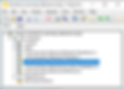
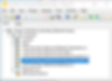
The following snippet shows the process of creating autoencoder's architecture (see the diagram above) with help of DeepLTK.

The input and the output sizes of the network are both 2000 samples. The blue sections in autoencoder diagram represent the fully connected (FC) layers, with their respective sizes indicated.
Front Panel of the Training VI
On the Front Panel of the Training VI, alongside all the common high-level configuration parameters, two additional graphs are presented on the right side: "Input & Reconstructed Signals" and "Anomaly Score", by which we can check the progress and accuracy during the training.

These graphs are being updated only when "Eval" button is pressed. "Input & Reconstructed Signals" graph shows the difference between the input and reconstructed signals. The input signal can be chosen from "Validation/Normal" or "Validation/Abnormal" datasets by toggling "Normal/Abnormal" boolean switch, and with help of the "Sample index" control we can chose a specific sample from the dataset.
The "Anomaly Score" graph visually represents the absolute difference between the input and reconstructed signals. Perfect performance of the network at train time implies that the anomaly score for normal samples converges to 0. In this context, a perfect match between the input and the reconstructed signal for normal samples results in an anomaly score equal to 0, indicating the model's precise ability to reconstruct the provided normal signal.
Training Process
Data Augmentation. As mentioned above, the input (training) dataset comprises of samples, which are randomly generated ideal sinusoidal signals. To enhance the model's learning capability, we introduce a small noise to the input samples at training time with help of augmentation parameters. These type of models are usually called denoising autoencoders and are used for training models which can remove the noise from the source signal, denoising application. But this is a topic for another day.

The addition of noise is implemented through the NN_Layer_Create(Input1D).vi.
In this specific case, we simply add uniform white noise with a magnitude of 2 to the input, which is very small compared to the 220v of amplitude of the input signal.
Let's execute the Training VI and observe how the training loss decreases over time.
Below is a video illustrating the training process.
As we aim for the model to learn the fundamental characteristics of normal signals, we desire the model to overfit. As it can be seen we are not using generalization parameters such as weight decays, to make sure the model is overfitting on the training dataset. The absence of such parameters ensures that the model focuses on memorizing the intricacies of the training dataset.
We also see that the Anomaly score for normal (training ) samples may not reach an ideal value of 0. This means, that we need to determine an anomaly score thresholdm, which is defined as follows. If the anomaly socre for a specific waveforme surpasses this threshold, it will indicate the presence of an anomaly in the signal. Conversely, if the score falls below the threshold, it signifies a normal signal.
Optimal Anomaly Score Threshold Evaluation
Now that our model is trained, the next step is to determine the right/optimal threshold to identify anomalies effectively. We have to identify the most suitable anomaly score threshold, where scores above indicate the presence of anomalies, while scores below signify normalcy.
We have created a separate VI to calculate the optimal threshold. "2_Anomaly_Threshold(Evaluation).vi" calculates the anomaly score threshold based on the model's performance on validation dataset which contains normal and abnormal amples.
First, using already trained model we calculate the maximum absolute difference between reconstructed and input signals and build histogram of anomaly score distribution both for normal and abnormal samples.
Depending on the performance of the model, or difficuilty of the task, we can have two posible distributions of anomaly scores. Namely teh histograms of normal and abnormal samples may be completely separated or can overlap, which is depicted in the picture below.

Now we have to find the most optimal threshold that optimally separates two distributions.
In the first case the task a relatively easy - we just need to chose a value between maximum of normal and minimum of abnormal distributions.
In the second case, when distributions overlap, we need to choose a threshold which lies somewhere in the vicinity of overlapping region. To find the optimal threshold, one of the criteria could be to maximize the number of correctly classified samples (i.e. the sum of True Positives (TP) and True Negatives (TN)).
To achieve this we are going to employ a technique called difference of integrals of distributions.
This method is described here on toy example of distributions depicted below.
Let's look at the two overlapped distributions:

As we told above we want to maximize correctly classified samples, by finding the optimal value of x, which can be defined as:

We know that:

Thus:

Note: The constant 1 is ignored, when finding the maximum.
The last row shows that we need to calculate the integrals of anomaly score distributions both for normal and abnormal datasets, calculate difference between them and find the argument at the maximum of this function.
For the case of overlapped distributions depicted in the picture above, the integrals of these distributions will be exactly as in the snapshot below.

By subtracting these integrals we will get the curve shown below:

As we can see, the graph has obvious maximum point (in case of non overlapping distributions,), which corresponds to optimal anomaly score threshold value. It should be noted, that this maximum, instead of point can become a region, if the distributions are non-overlapping.

This is the reason why the threshold is given with help of range, which becomes a point (Start = Stop ) for overlapping distributions.
Let's now have a look what kind of performance we can get on the problem of power transmission line anomaly detection.
For this we first use the Validation dataset to generate anomaly score prediction for normal and abnormal subsets to calculate optimal anomaly score threshold, which is depicted in the snapshot below.

As we can see the optimal value for anomaly score threshold is a range, because the trained model produces anomaly scores for normal and abnormal datasets, whos distributions are not overlapping. This means, that the model is capable of accurately learn features of normal signals, enabling the complete detection and separation of anomalies from normalcies. We will define as optimal threshold the center of this range, which is equal to 0.196.
Model Accuracy Evaluation
In the previous section, we used Validation dataset to find the optimal anomaly score threshold, which we will use here to measure model's accuracy on the Test dataset.

As it can be seen from the results with the threshold 0.196, the model is capable of classifying normal and abnormal samples with 100% of accuracy (Error Rate = 0).
Inference

Now as we have already quantitatively assessed the performance of the model, let's run some qualitative tests, by observing model's performance with interactively generating different data samples. This can be done with help of "4_WF_Anomaly_Detection(Inference).vi" and the process is depicted in the video below:
Conclusion
In conclusion, this blog post has provided a comprehensive guide on addressing waveform anomaly detection challenges using the DeepLTK. We have systematically navigated through the key stages of model development, including training, evaluation, and testing, to ensure robust performance and accuracy. By offering a step-by-step approach, this project serves as a valuable reference for individuals engaged in signal processing. Moreover, the adaptability of the provided example allows for easy customization to suit specific project requirements. Through the integration of DeepLTK and LabVIEW, users can efficiently tackle waveform anomaly detection tasks across a wide spectrum of applications within the field of signal processing.


